---
title: "Digits"
subtitle: "1,797 handwritten digits, 64d pixel vectors, k=10 ground truth."
order: 1
image: digits_files/figure-html/fig-dyf-output-1.png
categories: [images, small, pixels]
true-k: 10
format:
html:
code-fold: show
code-tools: true
execute:
warning: false
message: false
---
The smallest, fastest sanity check. `sklearn.datasets.load_digits` ships with the library — no downloads, runs in seconds, and the ground truth (`k=10`) is unambiguous. If DYF can't recover 10 groups here, nothing downstream matters.
It doesn't, quite. At the gallery defaults DYF recovers **7** groups for 10 classes — and the reason is the most useful thing this small dataset has to teach about how DYF works.
## Load the data
```{python}
#| label: load
from sklearn.datasets import load_digits

digits = load_digits()
X = digits.data.astype("float32")   # (1797, 64) — raw 8x8 pixel values
y = digits.target                   # (1797,) — integer class 0..9

print(f"{X.shape[0]} samples, {X.shape[1]}d, true k = {len(set(y))}")
```
## Run DYF (parameter-free)
Three lines. No `k`, no `eps`, no `min_cluster_size`. `_gallery.run_dyf` builds the tree with `build_dyf_tree`'s own defaults (`num_bits=3, max_depth=4, min_leaf_size=20`), the same on every notebook in this gallery — nothing is tuned per dataset.
```{python}
#| label: run-dyf
import sys
sys.path.insert(0, ".")
from _gallery import run_dyf, run_kmeans, run_hdbscan, plot_single, metrics_table

result = run_dyf(X, y)

print(f"Recovered k: {result.recovered_k}  (true k = {result.true_k})")
print(f"AMI:         {result.ami:.3f}")
print(f"ARI:         {result.ari:.3f}")
```
## Compare against k-means and HDBSCAN
```{python}
#| label: baselines
kmeans = run_kmeans(X, y)
hdb    = run_hdbscan(X, y)
```
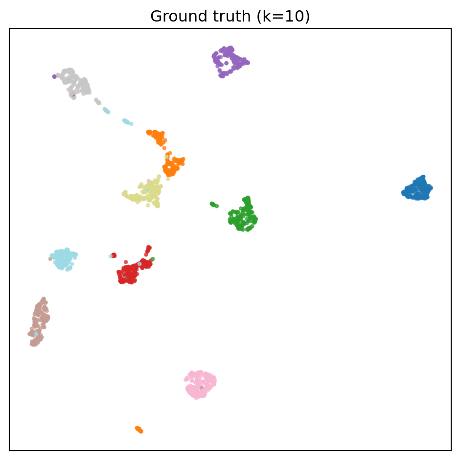
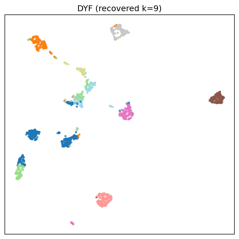
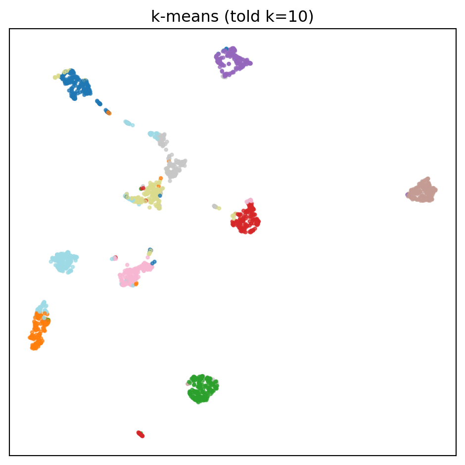
The same UMAP layout, coloured three different ways. Panels stack vertically, and on wider screens the layout tiles responsively (1→2→3 columns) via CSS `auto-fit`.
::: {.gallery-fluid}
```{python}
#| label: fig-truth
#| fig-cap: "Ground truth — each of the 10 digit classes."
plot_single(result.umap_2d, y, title=f"Ground truth (k={result.true_k})")
```
```{python}
#| label: fig-dyf
#| fig-cap: "DYF — parameter-free, no k supplied."
plot_single(result.umap_2d, result.labels, title=f"DYF (recovered k={result.recovered_k})")
```
```{python}
#| label: fig-kmeans
#| fig-cap: "K-means given the oracle k=10 (unfair ceiling)."
plot_single(result.umap_2d, kmeans["labels"], title=f"k-means (told k={result.true_k})")
```
:::
## Metrics
```{python}
#| label: metrics
#| output: asis
print(metrics_table(result, kmeans, hdb))
```
## How DYF and k-means disagree — and why
Squint at the three panels and the difference is obvious: **k-means's partitions track the ground-truth digit classes more faithfully than DYF's do.** K-means wins on every alignment metric here (AMI 0.77 vs 0.67, ARI 0.73 vs 0.54). That's worth being honest about.
Two things are driving the gap:
**1. The oracle is doing a lot of work.**
K-means was *told* `k=10`. That's not a small hint — it's the whole answer to the only question DYF actually has to solve. An algorithm with `k` handed to it is solving a completely different problem (a constrained one) than an algorithm that has to discover `k` from the data. The gallery exists precisely because you usually don't have that oracle.
**2. DYF under-splits here, and the reason is size.**
DYF does not cluster the 1,797 points directly. It builds a tree, takes the centroid of each leaf, and runs Louvain community detection on a k-nearest-neighbour graph of those centroids. On this dataset the tree has about 190 leaves. Modularity — the quantity Louvain maximises — has a well-known *resolution limit*: on a graph that small it cannot see communities below a certain size, and merges them. Two digit classes get absorbed into neighbours, and DYF reports 8.
That is not a property of the digits; it is a property of running a modularity optimiser on a 190-node graph at the standard resolution. The next cell shows the fix.
### Turning the one knob DYF actually has
`resolution` is the Louvain granularity parameter. At 1.0 (the default, used in every notebook) it under-splits this graph; at 2.0 it doesn't:
```{python}
#| label: run-dyf-res2
import tempfile
from pathlib import Path
import numpy as np
from sklearn.metrics import adjusted_mutual_info_score, adjusted_rand_score
from dyf import LazyIndex, build_dyf_tree, write_lazy_index
from dyf.agglomerate import louvain_cluster_leaves

tree = build_dyf_tree(X, seed=42, **result.tree_params)   # the same tree the page used
with tempfile.TemporaryDirectory() as td:
    path = str(Path(td) / "digits.dyf")
    write_lazy_index(tree, X, path, compression="none", quantization="float32")
    with LazyIndex(path) as idx:
        res2 = louvain_cluster_leaves(idx, result.umap_2d, X, resolution=2.0)
labels2 = np.asarray(res2.point_labels)

print(f"resolution=2.0 → recovered k: {len(set(labels2))}  "
      f"AMI: {adjusted_mutual_info_score(y, labels2):.3f}  "
      f"ARI: {adjusted_rand_score(y, labels2):.3f}")
```
Same tree, same leaves, one knob moved — and the count lands at the label's granularity with both metrics up. The gallery keeps `resolution=1.0` everywhere anyway, because no single value wins across the datasets (the large ones prefer 1–2, the small ones 2–4), and tuning it per dataset against the labels would defeat the point of the exercise. Read this cell as the diagnosis, not the recipe.
### Pros and cons, side by side
| | **DYF (parameter-free)** | **K-means (oracle k)** |
|-----------------------------------|-------------------------------------------------------------------------|----------------------------------------------------------------------------------------------|
| Needs `k`? | No — recovered from data. | Yes — given k=10 upfront. |
| Cluster shape | Arbitrary (density + graph connectivity). | Convex Voronoi cells around centroids. |
| Behavior when ground truth *is* convex blobs | Good once the tree has enough leaves; under-splits when it doesn't. | Excellent — this is exactly the geometry k-means optimizes for. |
| Behavior when ground truth is curved / elongated / nested | Follows the manifold; non-convex clusters are fine. | Fails — forces straight-line Voronoi cuts through curved structure. |
| Hierarchical output? | Yes — the tree gives you a multi-resolution structure for free. | No — flat partition at exactly `k`. |
| Sensitivity to ghost centers / init | Low — deterministic given seed. | High — `n_init` and `random_state` matter; can get stuck. |
### So why run DYF on digits at all?
Because the *story* of the gallery isn't "DYF beats k-means on every dataset." It's "DYF holds up *close enough* to oracle-tuned k-means on easy datasets, and pulls ahead where the oracle's assumptions break or the data gets big." Digits is the easy mode *and* the small mode — the one regime where DYF's leaf-centroid design is at a genuine disadvantage. [MNIST](mnist.qmd) is the same task at 40× the size, and there DYF beats oracle k-means on both metrics with the same defaults.
## What to take away
- **Recovered k** — DYF landed at 8 for 10. Below a few hundred leaves, expect this: the community-detection stage under-resolves small graphs at the default resolution. Above a few thousand leaves (MNIST, CIFAR) it lands on or next to the true count.
- **AMI** — the fairer comparison. K-means with the oracle *k* is the ceiling. DYF's gap to that ceiling is what you're paying for the privilege of not having to know *k* — and on this dataset, also for running a graph method on a tiny graph.
- **wall (s)** — at 1,797 points every method finishes in a few hundredths of a second, so the column says nothing here. It is on every page because it says something on the larger ones: DYF builds a tree, writes an index and runs Louvain, and that is slower than one k-means++ init wherever the gallery measured it.
- **HDBSCAN** — looks like a blowout when its AMI is reported in isolation, but note the `% discarded` column: HDBSCAN's defaults label a third of the points as *noise* on this dataset, and the AMI is computed only on the non-noise subset. It's answering a different question ("can you cluster the easy points?") than DYF and k-means ("can you cluster every point?").
## What this does not prove
- `load_digits` is a tiny, clean, well-separated dataset — the easy mode. The later notebooks (MNIST 70K, 20 Newsgroups, Olivetti) stress the same call under harder regimes.
- The pixel-space Euclidean metric on 8×8 images is kind to any clustering algorithm. The MNIST notebook repeats this on 70K samples at 28×28, where the geometry gets noticeably harder — and DYF gets noticeably better.
- Earlier versions of this page reported 9 communities and quoted AMI/ARI that did not match the cell output. The community counts before `dyf-rs` 0.12.0 came from a single-level Louvain that could not merge communities (dyf `KNOWN_ISSUES.md`, issue 10); the numbers here are from the corrected optimiser.