MNIST

70,000 handwritten digits, 28×28 pixel vectors, k=10 ground truth.

The scaled-up version of Digits. Same domain, same task, same k=10 — but 40× more samples and 12× higher pixel dimensionality. Does DYF’s parameter-free story survive the jump in scale, or does it fall apart under a heavier load?

Short answer, as we’ll see: it gets better with scale. On Digits, oracle k-means beat DYF on both metrics. On MNIST, DYF — told nothing — recovers 12 communities for 10 classes and beats oracle k-means on both AMI and ARI. The reason is worth understanding, because it is the same reason DYF under-performs on the small dataset.

Load MNIST

import os
import numpy as np

CACHE = "/tmp/gallery_mnist.npz"
if os.path.exists(CACHE):
    z = np.load(CACHE)
    X, y = z["X"], z["y"]
else:
    from sklearn.datasets import fetch_openml
    m = fetch_openml("mnist_784", version=1, as_frame=False, parser="auto")
    X = (m.data.astype(np.float32) / 255.0)   # normalize pixels to [0, 1]
    y = m.target.astype(int)
    np.savez(CACHE, X=X, y=y)

print(f"{X.shape[0]:,} samples, {X.shape[1]}d, true k = {len(set(y))}")

70,000 samples, 784d, true k = 10

Run DYF

import sys
sys.path.insert(0, ".")
from _gallery import run_dyf_cached, run_kmeans, plot_single, metrics_table

result = run_dyf_cached(X, y, cache_path="/tmp/gallery_mnist_dyf.npz")
print(f"Recovered k: {result.recovered_k}  (true k = {result.true_k})")
print(f"AMI:         {result.ami:.3f}")
print(f"ARI:         {result.ari:.3f}")

Recovered k: 12  (true k = 10)
AMI:         0.546
ARI:         0.422

Oracle k-means

kmeans = run_kmeans(X, y)
print(f"k-means AMI={kmeans['ami']:.3f}, ARI={kmeans['ari']:.3f} (told k={result.true_k})")

k-means AMI=0.491, ARI=0.361 (told k=10)

Figures

plot_single(result.umap_2d, y, title=f"Ground truth (k={result.true_k})")

Figure 1: Ground truth — each of the 10 digit classes.

plot_single(result.umap_2d, result.labels, title=f"DYF (recovered k={result.recovered_k})")

Figure 2: DYF — parameter-free, no k supplied.

plot_single(result.umap_2d, kmeans["labels"], title=f"k-means (told k={result.true_k})")

Figure 3: K-means given the oracle k=10.

Metrics

print(metrics_table(result, kmeans, None))

Method	Recovered k	AMI	ARI	% discarded	wall (s)
DYF (parameter-free)	12	0.546	0.422	0%	8.19
k-means (oracle k=10)	10	0.491	0.361	0%	1.22

Wall time: DYF 8.19 s (tree build + index write + Louvain) vs k-means 1.22 s (one k-means++ init at the oracle k) — DYF 6.7× slower here. The shared UMAP layout is not counted for either.

This is also the first page where the wall (s) column matters. DYF is the slower tool: a tree over 70,000 × 784 rows, a written index and a Louvain pass cost several times one k-means++ init at k=10. What that time buys is in the next two sections — a partition that beats the oracle, and a hierarchy under it that k-means cannot produce at any k. The regime where DYF is the faster tool is a different comparison: at 1.3M cells it matches a kNN-graph + Leiden pipeline’s partition in a fraction of the time (dyf KNOWN_ISSUES.md #10), and that pipeline, not k-means, is what people run at that scale.

Deep dive: where do DYF’s 12 clusters come from?

Twelve clusters for ten digits is close enough to the label’s own granularity that the interesting question is no longer “why so many?” but “which two digits got split, and did anything get merged?” This section answers both from the partition itself.

First, the statistical audit

If DYF’s clusters track the digit classes, each should be dominated by one digit. Mixed bags are the signature of classes being merged.

import numpy as np
from collections import Counter

labels = result.labels
rows = []
for cid in sorted(set(labels)):
    mask = labels == cid
    n = int(mask.sum())
    if n == 0:
        continue
    vals, cnts = np.unique(y[mask], return_counts=True)
    rows.append({"cid": cid, "n": n, "dominant": int(vals[np.argmax(cnts)]),
                 "purity": cnts.max() / n})

r80 = sum(1 for r in rows if r["purity"] > 0.80)
r90 = sum(1 for r in rows if r["purity"] > 0.90)
r95 = sum(1 for r in rows if r["purity"] > 0.95)
weighted = sum(r["purity"] * r["n"] for r in rows) / sum(r["n"] for r in rows)

digit_counts = Counter(r["dominant"] for r in rows)
per_digit = ", ".join(f"{d}×{n}" for d, n in sorted(digit_counts.items()))

print(f"**{len(rows)} DYF clusters. Weighted purity: {weighted:.3f}.**\n")
print(f"- {r80}/{len(rows)} clusters are >80% pure (dominated by one digit)\n")
print(f"- {r90}/{len(rows)} are >90% pure\n")
print(f"- {r95}/{len(rows)} are >95% pure\n")
print(f"- Clusters per digit: {per_digit}\n")

12 DYF clusters. Weighted purity: 0.643.

• 4/12 clusters are >80% pure (dominated by one digit)

• 2/12 are >90% pure

• 0/12 are >95% pure

• Clusters per digit: 0×1, 1×1, 2×1, 3×2, 4×1, 5×1, 6×2, 7×1, 8×1, 9×1

Every digit has at least one cluster where it is the majority, so nothing was lost outright. But a weighted purity around two-thirds says several clusters are shared between digits. The next cell names them.

Split digits and merged digits

by_digit = {}
for r in rows:
    by_digit.setdefault(r["dominant"], []).append(r)
split = {d: sorted(rs, key=lambda r: -r["n"]) for d, rs in by_digit.items() if len(rs) > 1}
mixed = sorted([r for r in rows if r["purity"] < 0.6], key=lambda r: -r["n"])

print(f"**Digits split across more than one DYF cluster:** {', '.join(str(d) for d in sorted(split)) or 'none'}\n")
for d, rs in sorted(split.items()):
    print(f"- digit {d}: " + "; ".join(f"cluster {r['cid']} (n={r['n']:,}, {r['purity']:.0%} {d}s)" for r in rs) + "\n")

print(f"\n**Clusters with no dominant digit (purity < 60%):** {len(mixed)}\n")
for r in mixed:
    mask = labels == r["cid"]
    vals, cnts = np.unique(y[mask], return_counts=True)
    order = np.argsort(-cnts)[:3]
    print(f"- cluster {r['cid']} (n={r['n']:,}): " + ", ".join(f"{int(vals[i])} {cnts[i] / r['n']:.0%}" for i in order) + "\n")

# For the image grids below: the split digit whose two largest sub-clusters are purest.
show_digit = max(split, key=lambda d: min(r["purity"] for r in split[d][:2])) if split else None
show_subs = split[show_digit][:2] if show_digit is not None else []

Digits split across more than one DYF cluster: 3, 6

• digit 3: cluster 9 (n=5,968, 38% 3s); cluster 2 (n=5,813, 66% 3s)

• digit 6: cluster 8 (n=4,643, 80% 6s); cluster 11 (n=3,899, 71% 6s)

Clusters with no dominant digit (purity < 60%): 5

• cluster 1 (n=8,160): 4 44%, 9 42%, 7 5%

• cluster 3 (n=7,496): 9 34%, 7 32%, 4 28%

• cluster 5 (n=6,696): 8 53%, 1 27%, 2 8%

• cluster 9 (n=5,968): 3 38%, 5 29%, 8 24%

• cluster 4 (n=4,722): 5 56%, 0 21%, 8 10%

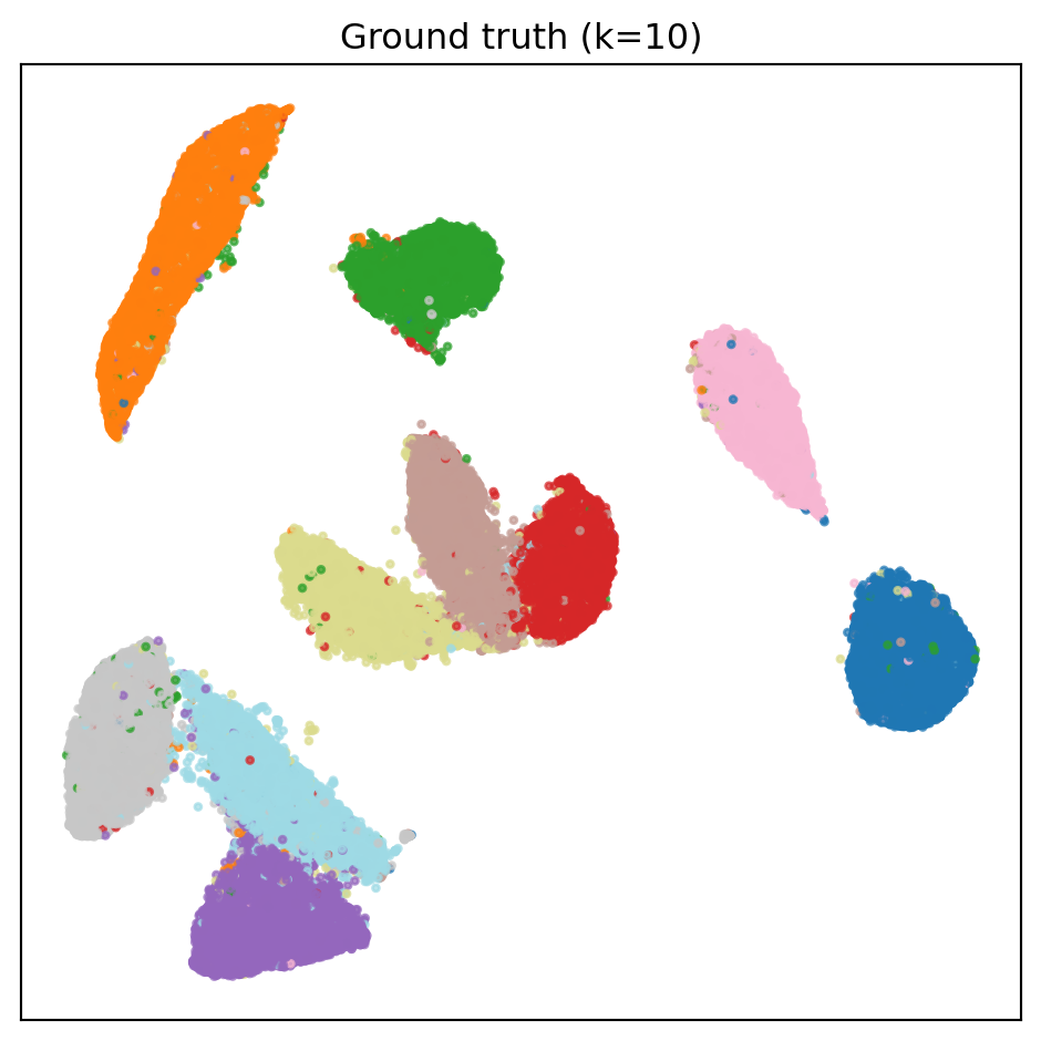
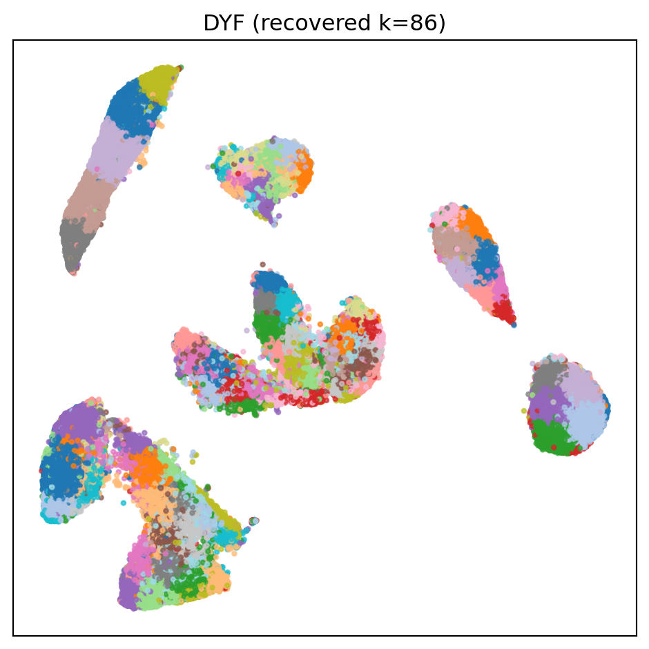
Read the two lists together. The two “extra” clusters are the digit 6 split into two near-equal halves, each about 80% pure — that is the split the pictures below examine. The digit 3 is also split, but one of its halves is really a 3/5/8 mixture. And the impurity has one dominant source: 4 and 9 are never separated — they share two clusters, each roughly 40% fours and 40% nines — with 8-with-1 and 5-with-0 as smaller confusions. In pixel space a closed-top 4 and a 9 are a few pixels apart, so this is the classic MNIST confusion showing up as a merge rather than as misclassification. Nothing here is a class fragmented into arbitrary pieces; every decision is one the flat label cannot express, and the pictures decide whether the one clean split is sensible.

The split digit, as images

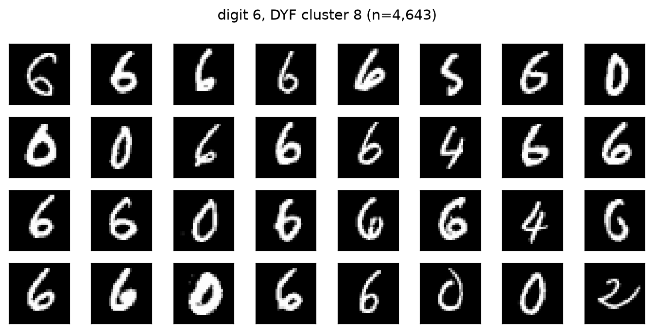
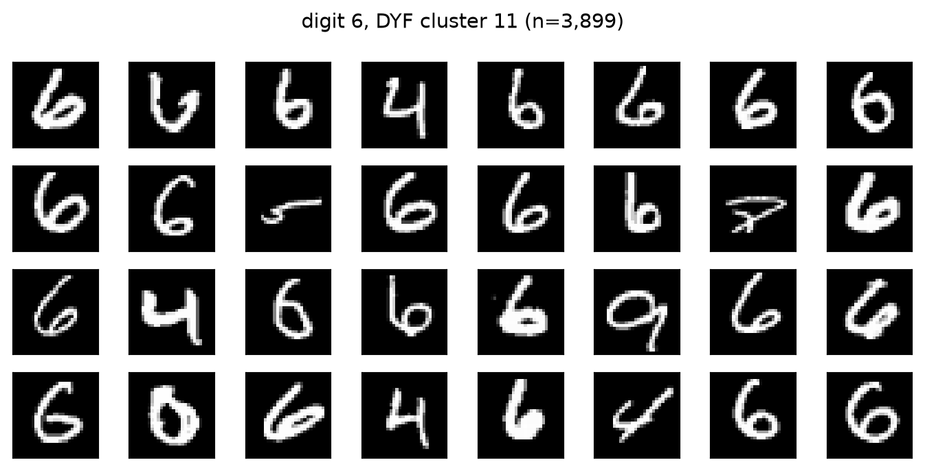
The digit below is the one DYF divided most cleanly into two communities. Each grid is a random sample from one of them:

from _gallery import image_grid
fig_a = None
if len(show_subs) >= 1:
    idx = np.where(result.labels == show_subs[0]["cid"])[0]
    fig_a = image_grid(X, idx, title=f"digit {show_digit}, DYF cluster {show_subs[0]['cid']} (n={show_subs[0]['n']:,})")
fig_a  # a bare expression displays; a call inside the `if` would not

Figure 4: DYF sub-cluster A of the split digit — random sample.

fig_b = None
if len(show_subs) >= 2:
    idx = np.where(result.labels == show_subs[1]["cid"])[0]
    fig_b = image_grid(X, idx, title=f"digit {show_digit}, DYF cluster {show_subs[1]['cid']} (n={show_subs[1]['n']:,})")
fig_b

Figure 5: DYF sub-cluster B of the same digit — random sample.

Two ways of writing a 6. The first grid’s sixes have a small, tight loop on a long stem, mostly thin and slanted; the second grid’s have a large round loop and heavier strokes — and its impurities are 0s, which is what a big-looped 6 turns into when the stem shortens. It is a difference of loop size and stroke weight rather than two unmistakably different populations, so read it as a stylistic sub-community the ten-way label has no room for: modest, visible, and the kind of split a retrieval task would want kept. The caveats say how we’d test that properly.

The same digit, from k-means

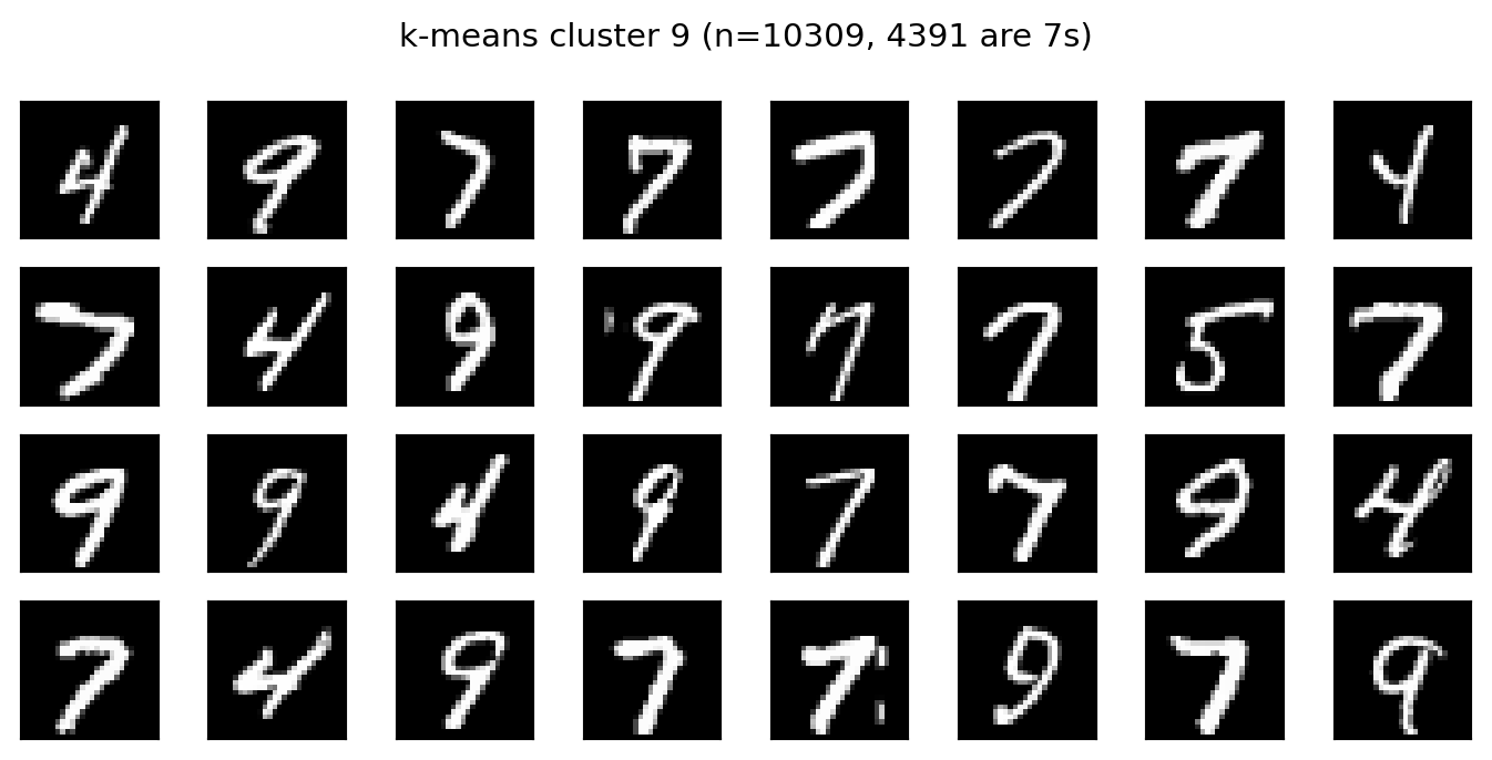
K-means was told k=10, so it gave us exactly ten clusters. Here’s a random sample from the cluster that contains the most 7s:

km_labels = kmeans["labels"]
best_cid, best_count = -1, 0
for cid in np.unique(km_labels):
    cnt = int(((km_labels == cid) & (y == 7)).sum())
    if cnt > best_count:
        best_count, best_cid = cnt, int(cid)
idx = np.where(km_labels == best_cid)[0]
image_grid(X, idx, title=f"k-means cluster {best_cid} (n={len(idx):,}, {best_count:,} are 7s)")

Figure 6: The k-means cluster that contains the most 7s.

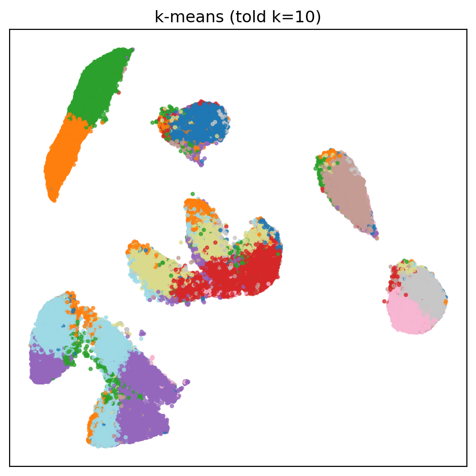
Read the title: the fraction of this cluster that is actually a 7. The rest are other digits — mostly 4s, 9s and 5s — that share a prominent diagonal stroke in pixel space. Committing to exactly ten Voronoi cells forced k-means to draw a boundary somewhere, and “things with a diagonal stroke” was the cleanest cut available. DYF spent its budget differently: it kept the digit classes apart and used two extra clusters on a style split. That is why it wins ARI here as well as AMI.

Why this matters

If your downstream task is classification (given a new image, predict 0–9), you want a ten-way partition — and on MNIST the one DYF finds without being told k is closer to the labels than the one k-means finds with it.

If your downstream task is retrieval (given a user’s handwriting, find visually similar samples), the style split is the feature you want kept.

If your downstream task is exploration (what’s in this corpus?), you want the hierarchy: start at the 12 communities, then walk down to 10 or 5 to see how they merge, without refitting.

Walking down the hierarchy

DYF’s 12 communities sit at the top of a partition hierarchy. merge_to_max_k collapses them to coarser granularities:

from _gallery import merge_walk, merge_walk_table

walk = merge_walk(result, X, y, targets=[40, 20, 10, 5])
print(merge_walk_table(walk, result))

Resolution	Actual k	AMI	ARI
Raw DYF	12	0.546	0.422
merge → 40	12	0.546	0.422
merge → 20	12	0.546	0.422
merge → 10	10	0.500	0.363
merge → 5	5	0.399	0.275

Targets above 12 are no-ops — there is nothing to merge. Merging to exactly 10 costs a little on both metrics, because the two extra clusters were a real split and forcing them back together is the wrong merge for this label. The raw partition is the best point on the walk. That is what “recover k from the data” looks like when it works: the finest natural partition is already at the label’s granularity, and the walk is there for the tasks that want something coarser.

What happened to the Digits story?

The two datasets tell opposite stories, and the comparison is the most instructive table in the gallery:

Dataset	DYF k	k-means AMI	DYF AMI	DYF − k-means AMI	DYF ARI	k-means ARI
Digits	8	0.773	0.668	−0.105	0.536	0.726
MNIST	12	0.491	0.546	+0.055	0.422	0.361

On 1,797 digits DYF under-splits (8 communities for 10 classes) and loses on both metrics. On 70,000 it lands at 12 and wins on both. Same code, same defaults.

Why does scale help?

DYF clusters leaf centroids, not points. On Digits the tree has around 190 leaves; a modularity optimiser on a graph that small hits its resolution limit and merges genuine classes — the well-known failure of modularity on small graphs, not a property of the digits. On MNIST the tree has about 3,200 leaves, the community graph is rich enough to resolve ten-plus communities, and the partition snaps to the label. The Digits notebook shows the other side of this: raising the Louvain resolution to 2 recovers 10 communities there and beats the default on both metrics.

So the axis that matters is not sample count as such but leaf count — how many super-points the tree hands to community detection. Below a few hundred, expect under-splitting at the default resolution.

The sports analogy update

Digits was k-means’s home court — convex blobs, small k, oracle-provided, and a DYF that could not field enough players. It won cleanly.

MNIST is the away game with a full roster. K-means still had the oracle, and still lost on both scoreboards — because knowing k=10 does not tell you where to cut, and pixel space rewarded the cut that keeps digit classes apart over the one that hits exactly ten centers.

Caveats

• The two extra clusters need a look, not a number. The grids above are the evidence. Our reading is that the split is stylistic (reading (a)); a rigorous version would test it by holding out the split digit and checking whether the two sub-clusters predict, say, writer identity or stroke width. The gallery skips that to keep the notebook readable.
• Earlier versions of this page reported 81–86 DYF clusters and built an “over-partitioning is hierarchy” argument on them. That count was an artifact: the Louvain optimiser in dyf-rs before 0.12.0 ran a single level with no aggregation phase and could not merge communities once formed. The fix is documented in dyf’s KNOWN_ISSUES.md (issue 10); the numbers on this page are from the corrected optimiser.
• UMAP is a projection, not the cluster space. When DYF’s and k-means’s partitions look visually different in the UMAP panel, some of that is true clustering difference and some is UMAP’s 2D compression of decisions made in 784d. Don’t read the UMAP too literally.
• Cache is in /tmp. Dumped on reboot, which is fine for the gallery — real applications should use a durable cache.