---
title: "Synthetic Shapes"
subtitle: "Moons, circles, and varied-density blobs — where DYF is not the best tool, and why that's OK."
order: 0
image: synthetic-shapes_files/figure-html/fig-moons-dyf-output-1.png
categories: [synthetic, 2d, pedagogical]
true-k: "2–5"
format:
html:
code-fold: show
code-tools: true
execute:
warning: false
message: false
---
Before this notebook, I was going to tell you DYF handles curved non-convex shapes well. The tests I ran told a different, more useful story: **on low-dimensional toy shapes, HDBSCAN beats DYF decisively — and the right conclusion isn't to pretend otherwise, it's to understand *when* each method earns its keep.**
This notebook runs all three methods (DYF, HDBSCAN, and oracle-k k-means) on three canonical synthetic datasets. HDBSCAN wins every one. The point isn't that DYF is bad; it's that DYF's value prop lives at scales and dimensionalities where HDBSCAN itself starts to struggle — which is what the real-world notebooks in this gallery show.
## Shape 1: Two moons
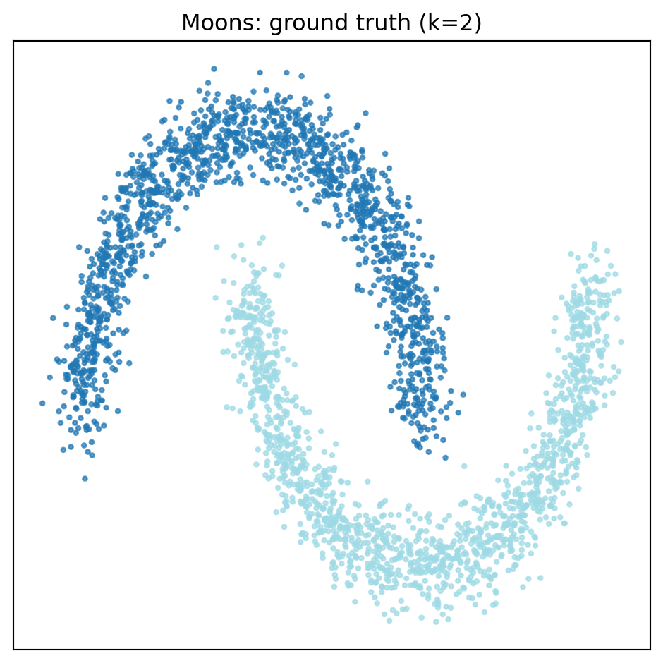
Two interleaved crescents. The textbook "k-means fails, density-based methods succeed" case.
```{python}
#| label: moons-run
import sys
sys.path.insert(0, ".")
import numpy as np
from sklearn.datasets import make_moons
from _gallery import run_dyf, run_kmeans, run_hdbscan, plot_single

X, y = make_moons(n_samples=3000, noise=0.08, random_state=42)
X = X.astype(np.float32)
r_moons   = run_dyf(X, y)
km_moons  = run_kmeans(X, y)
hdb_moons = run_hdbscan(X, y)

print(f"DYF       k={r_moons.recovered_k}       AMI={r_moons.ami:.3f} ARI={r_moons.ari:.3f}  wall={r_moons.seconds:.2f}s")
print(f"k-means   told k=2  AMI={km_moons['ami']:.3f} ARI={km_moons['ari']:.3f}  wall={km_moons['seconds']:.2f}s")
print(f"HDBSCAN   k={hdb_moons['recovered_k']} noise={hdb_moons['noise_frac']:.1%}  AMI={hdb_moons['ami']:.3f} ARI={hdb_moons['ari']:.3f}  wall={hdb_moons['seconds']:.2f}s")
```
::: {.gallery-fluid}
```{python}
#| label: fig-moons-truth
#| fig-cap: "Ground truth — two crescents."
plot_single(X, y, title="Moons: ground truth (k=2)")
```
```{python}
#| label: fig-moons-dyf
#| fig-cap: "DYF partially follows the shape but splits one moon in half."
plot_single(X, r_moons.labels, title=f"Moons: DYF (k={r_moons.recovered_k})")
```
```{python}
#| label: fig-moons-hdb
#| fig-cap: "HDBSCAN — perfect separation, 0.2% noise."
plot_single(X, hdb_moons["labels"], title=f"Moons: HDBSCAN (k={hdb_moons['recovered_k']})")
```
```{python}
#| label: fig-moons-kmeans
#| fig-cap: "K-means — straight-line cut bisects both crescents."
plot_single(X, km_moons["labels"], title="Moons: k-means (told k=2)")
```
:::
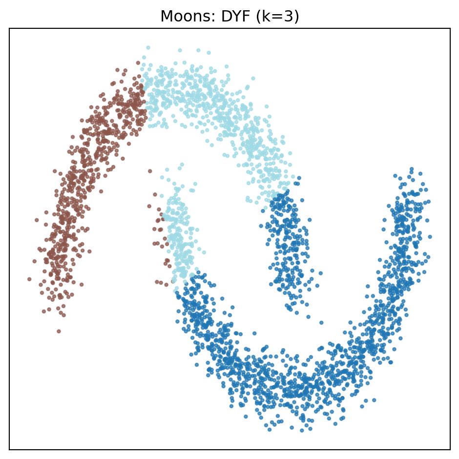
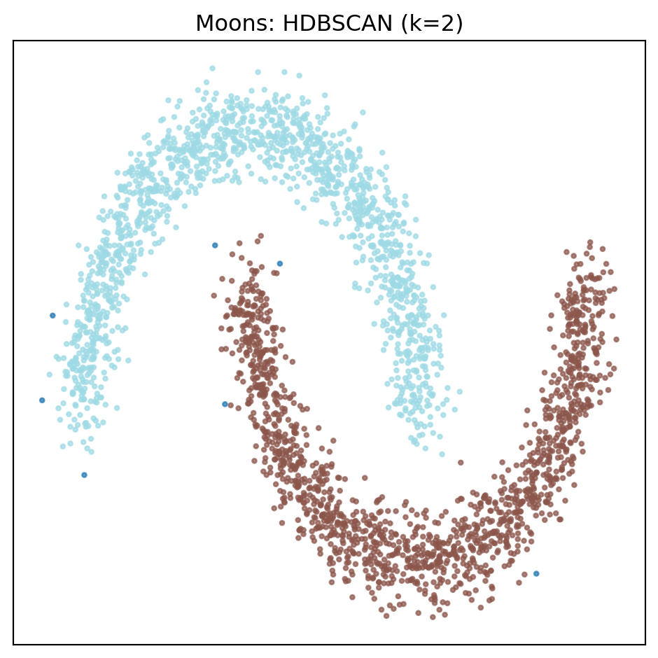
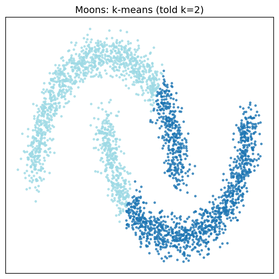
**HDBSCAN nails this perfectly (AMI=ARI=1.000).** DYF modestly beats k-means but splits one crescent into two clusters — a crosstab against ground truth shows DYF's largest cluster is 83% moon-1, a middle cluster is 97% moon-0, and the third is 76% moon-0 with bleeder points. It's not "following the crescents" — it's doing LSH hyperplane splits that happen to correlate with the ground truth.
Why does HDBSCAN beat DYF here? HDBSCAN uses *mutual reachability* distances — it literally follows density ridges through the data, tracking connected-density regions. That's the right tool for a curved 2D manifold. DYF's mechanism is different: recursive LSH splits → leaf centroids → Louvain on the centroid KNN graph. That's designed for *scale*, not *shape*. The 2D regime is HDBSCAN's turf.
### And the merge walk can't rescue it
DYF's multi-resolution pitch — [seen on MNIST](mnist.qmd#walking-down-the-hierarchy) and [20 Newsgroups](twenty-newsgroups.qmd#walking-down-the-hierarchy) — is that you can walk down the partition hierarchy to coarser resolutions post-hoc. On moons, merging DYF's k=3 output down to k=2 produces:
```{python}
#| label: moons-merge
#| output: asis
from _gallery import merge_walk, merge_walk_table
print(merge_walk_table(merge_walk(r_moons, X, y, targets=[2]), r_moons))
```
AMI *decreases* from 0.323 to 0.258. The merge walk assumes the raw over-partition contains the coarser structure as a sub-partition — when it doesn't (because the original LSH cuts went *across* the ground truth), merging just averages the wrong fragments together. **Merging walks hierarchy; it doesn't fix geometry.** This is the honest failure mode to contrast against MNIST, where the raw 12-way partition is already the best point on the walk and every merge costs a little on both metrics.
## Shape 2: Concentric circles
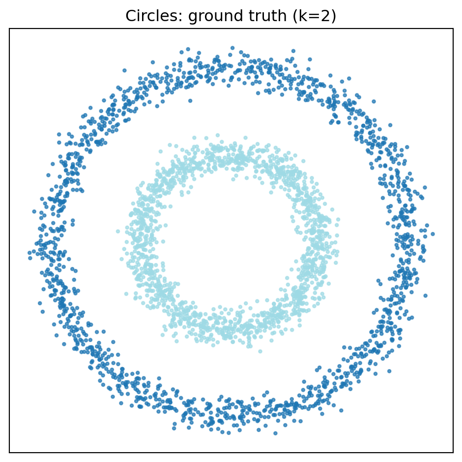
Inner ring nested inside outer ring. This is traditionally described as a spectral-clustering problem, because neither k-means nor classic density methods are supposed to handle topological nesting. Let's check.
```{python}
#| label: circles-run
from sklearn.datasets import make_circles

X, y = make_circles(n_samples=3000, noise=0.05, factor=0.5, random_state=42)
X = X.astype(np.float32)
r_circ   = run_dyf(X, y)
km_circ  = run_kmeans(X, y)
hdb_circ = run_hdbscan(X, y)

print(f"DYF       k={r_circ.recovered_k}       AMI={r_circ.ami:.3f} ARI={r_circ.ari:.3f}  wall={r_circ.seconds:.2f}s")
print(f"k-means   told k=2  AMI={km_circ['ami']:.3f} ARI={km_circ['ari']:.3f}  wall={km_circ['seconds']:.2f}s")
print(f"HDBSCAN   k={hdb_circ['recovered_k']} noise={hdb_circ['noise_frac']:.1%}  AMI={hdb_circ['ami']:.3f} ARI={hdb_circ['ari']:.3f}  wall={hdb_circ['seconds']:.2f}s")
```
::: {.gallery-fluid}
```{python}
#| label: fig-circles-truth
#| fig-cap: "Ground truth — inner ring nested inside outer."
plot_single(X, y, title="Circles: ground truth (k=2)")
```
```{python}
#| label: fig-circles-dyf
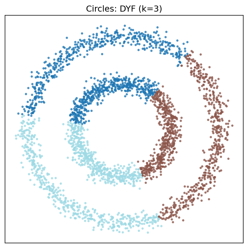
#| fig-cap: "DYF — cuts by angle, misses the nesting."
plot_single(X, r_circ.labels, title=f"Circles: DYF (k={r_circ.recovered_k})")
```
```{python}
#| label: fig-circles-hdb
#| fig-cap: "HDBSCAN — separates the rings cleanly."
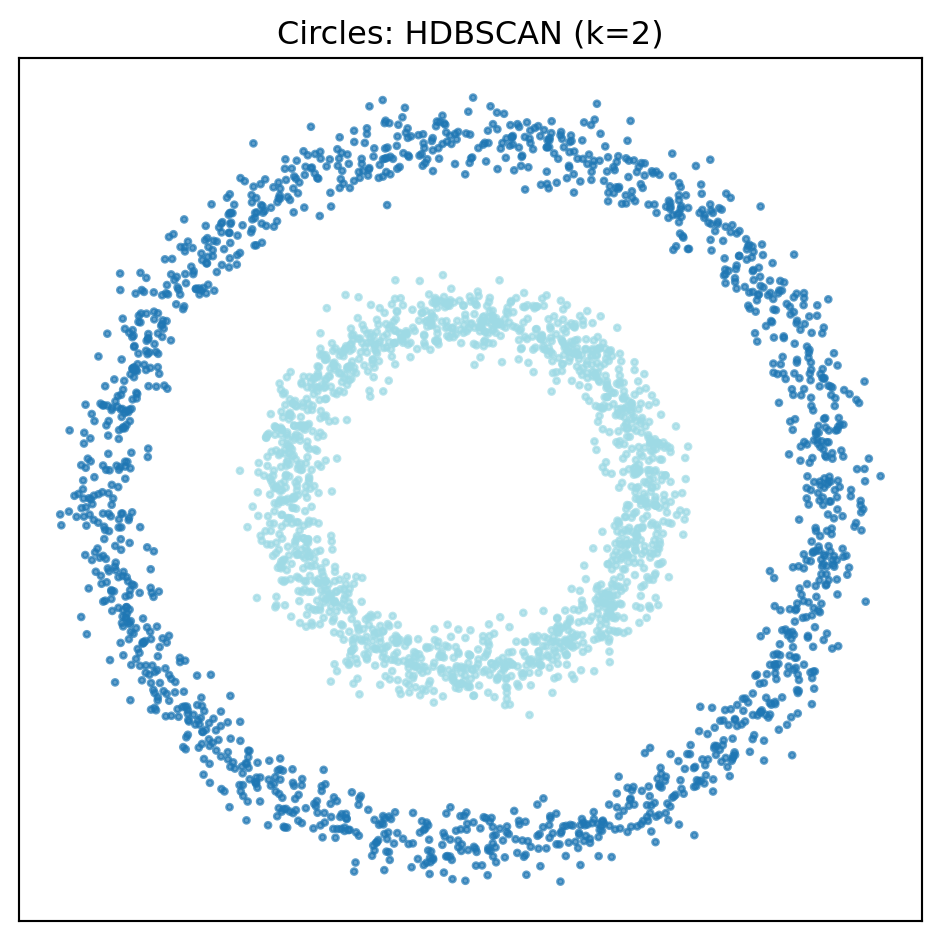
plot_single(X, hdb_circ["labels"], title=f"Circles: HDBSCAN (k={hdb_circ['recovered_k']})")
```
```{python}
#| label: fig-circles-kmeans
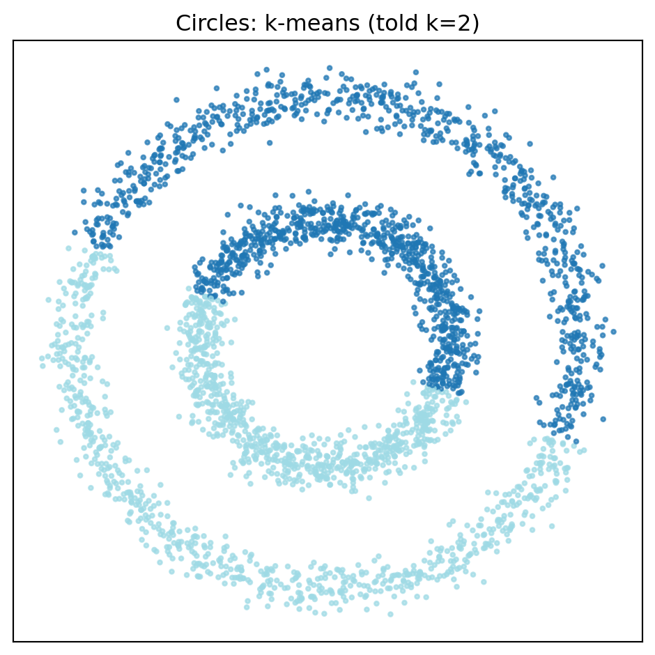
#| fig-cap: "K-means — same angular failure as DYF."
plot_single(X, km_circ["labels"], title="Circles: k-means (told k=2)")
```
:::
**Both DYF and k-means score AMI ≈ 0. HDBSCAN scores AMI=1.000.** The conventional wisdom — *"concentric rings require spectral clustering"* — turns out to be overstated. HDBSCAN handles them because the *gap between the rings* is a density valley, and HDBSCAN's mutual-reachability metric picks that gap up as a cluster boundary. DYF, which cuts by LSH hyperplane rather than by density valley, cannot see the gap.
## Shape 3: Varied-density blobs
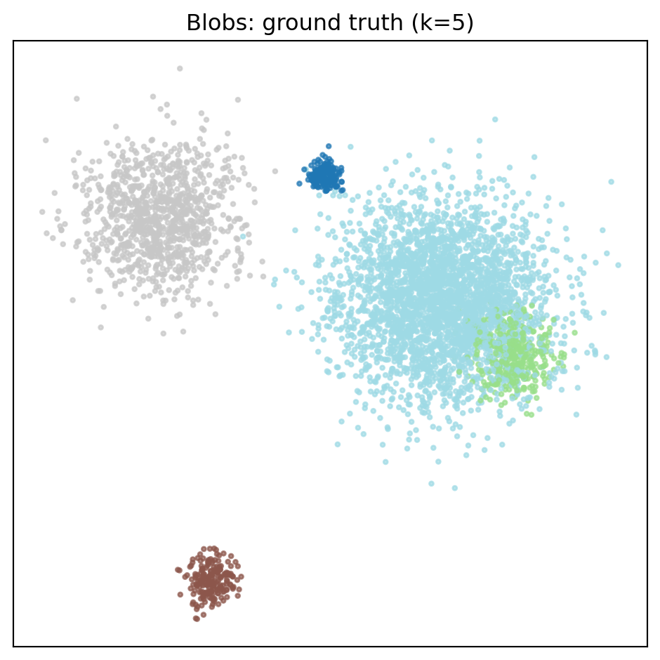
Five Gaussians with unequal sample sizes and spreads: `[200, 400, 200, 1000, 3000]` samples at `[0.3, 0.8, 0.5, 1.5, 2.0]` std. Uneven density is where parameter-free methods traditionally disagree.
```{python}
#| label: blobs-run
from sklearn.datasets import make_blobs

X, y = make_blobs(
    n_samples=[200, 400, 200, 1000, 3000],
    cluster_std=[0.3, 0.8, 0.5, 1.5, 2.0],
    n_features=2,
    random_state=42,
)
X = X.astype(np.float32)
r_blobs   = run_dyf(X, y)
km_blobs  = run_kmeans(X, y)
hdb_blobs = run_hdbscan(X, y)

print(f"DYF       k={r_blobs.recovered_k}       AMI={r_blobs.ami:.3f} ARI={r_blobs.ari:.3f}  wall={r_blobs.seconds:.2f}s")
print(f"k-means   told k=5  AMI={km_blobs['ami']:.3f} ARI={km_blobs['ari']:.3f}  wall={km_blobs['seconds']:.2f}s")
print(f"HDBSCAN   k={hdb_blobs['recovered_k']} noise={hdb_blobs['noise_frac']:.1%}  AMI={hdb_blobs['ami']:.3f} ARI={hdb_blobs['ari']:.3f}  wall={hdb_blobs['seconds']:.2f}s")
```
::: {.gallery-fluid}
```{python}
#| label: fig-blobs-truth
#| fig-cap: "Ground truth — five blobs, varied sizes and spreads."
plot_single(X, y, title="Blobs: ground truth (k=5)")
```
```{python}
#| label: fig-blobs-dyf
#| fig-cap: "DYF — under-partitions, merges diffuse blobs."
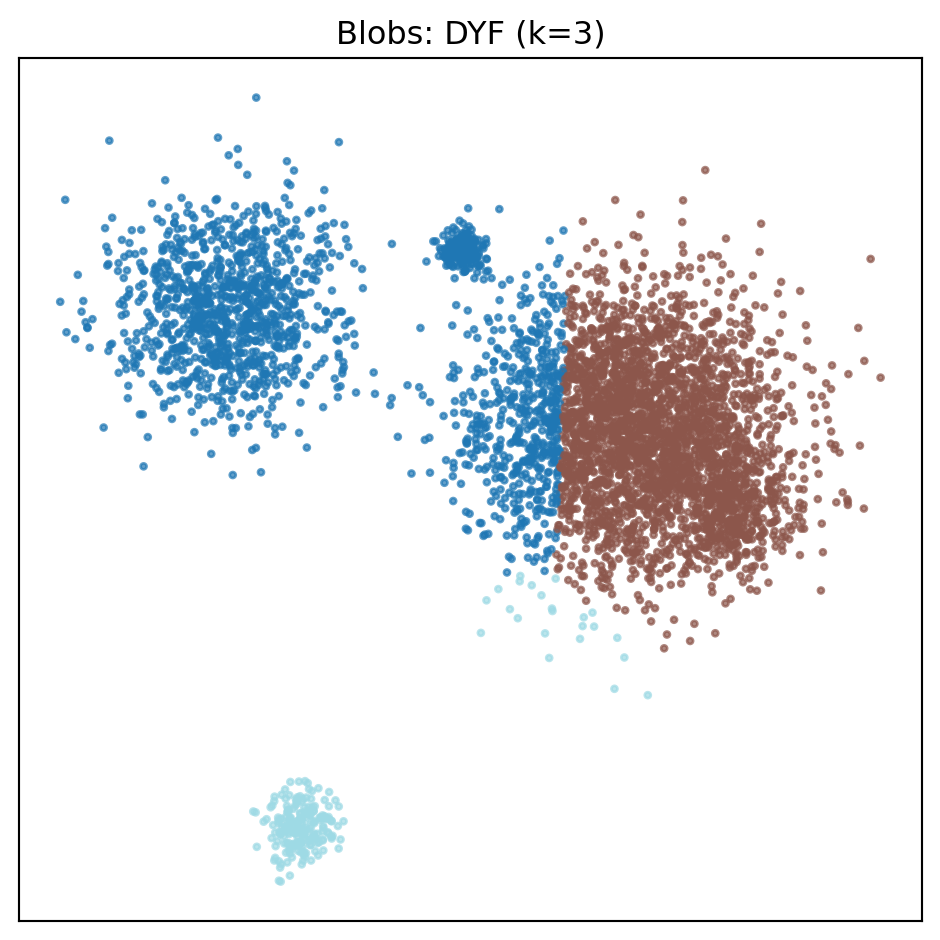
plot_single(X, r_blobs.labels, title=f"Blobs: DYF (k={r_blobs.recovered_k})")
```
```{python}
#| label: fig-blobs-hdb
#| fig-cap: "HDBSCAN — finds 5 clusters with minimal noise."
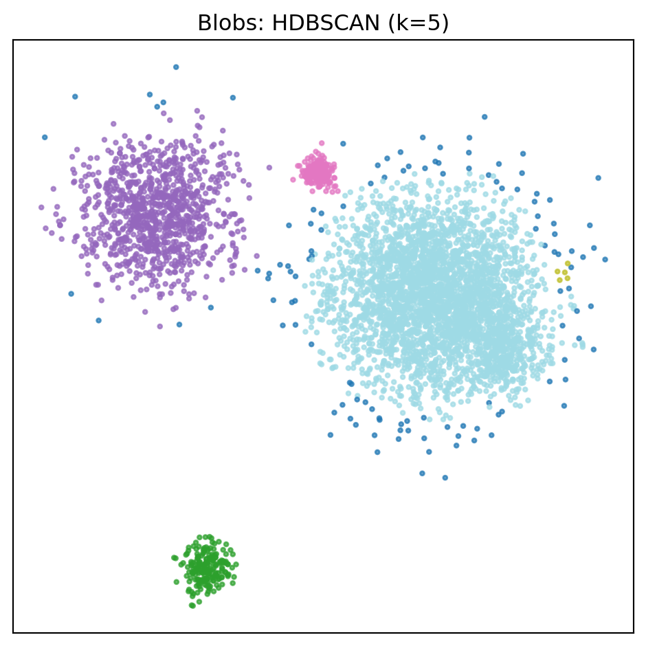
plot_single(X, hdb_blobs["labels"], title=f"Blobs: HDBSCAN (k={hdb_blobs['recovered_k']})")
```
```{python}
#| label: fig-blobs-kmeans
#| fig-cap: "K-means — correct k, noisy borders between tight and diffuse blobs."
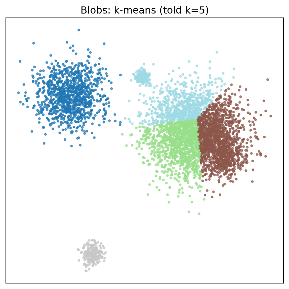
plot_single(X, km_blobs["labels"], title="Blobs: k-means (told k=5)")
```
:::
HDBSCAN again wins — 5 clusters with 2.5% noise, AMI=0.853. DYF under-partitions to 3 clusters. The metric tradeoff between under- and over-partitioning is still worth noting:
| Dataset | DYF recovered_k | vs true | DYF AMI vs kmeans | DYF ARI vs kmeans |
|---------|----------------:|---------|------------------:|------------------:|
| MNIST | 12 | 20% over | DYF +0.055 | DYF +0.061 |
| Blobs | 3 | 40% under | DYF **−0.102** | DYF +0.091 |
**Under-partitioning splits the metrics** — against k-means, DYF loses AMI and wins ARI on Blobs. (An earlier version of this page set that against a mirror image on MNIST, where an 81-cluster over-partition won AMI and lost ARI; that count was the single-level Louvain artifact of dyf `KNOWN_ISSUES.md` #10, and the corrected optimiser's 12 clusters win both.) AMI and ARI still weigh the two directions of error differently; read them together.
## Summary
| Shape | HDBSCAN | DYF | k-means (oracle) | Best tool |
|----------|---------|-----|------------------|-----------|
| Moons | **1.000** / 1.000 | 0.323 / 0.350 | 0.192 / 0.254 | **HDBSCAN** |
| Circles | **1.000** / 1.000 | 0.000 / 0.000 | 0.000 / 0.000 | **HDBSCAN** |
| Blobs | **0.853** / 0.785 | 0.524 / 0.444 | 0.626 / 0.353 | **HDBSCAN** |
HDBSCAN wins cleanly on all three. So why is DYF in the gallery at all?
## Why HDBSCAN isn't in every other notebook
Because HDBSCAN's synthetic-shape performance doesn't generalize. On the real-world notebooks — [Digits](digits.qmd), [20 Newsgroups](twenty-newsgroups.qmd), [CIFAR-10 + CLIP](cifar10-clip.qmd), [CMU MoCap](cmu-mocap.qmd) — HDBSCAN starts to break:
- **Digits (1,797 × 64d)**: HDBSCAN labels most points as noise. Its 0.935 AMI is computed on only the 40% of points it was willing to cluster; the other 60% got `-1`. That's not an honest apples-to-apples comparison with methods that partition every point.
- **20 Newsgroups (18,846 × 384d)**: HDBSCAN takes 144 seconds of wall clock and discards 84% of posts as noise. The real-world notebook documents this and omits HDBSCAN from the comparison because it's not usable at that scale.
- **CIFAR-10 (10,000 × 512d)** and **MNIST (70,000 × 784d)**: HDBSCAN's runtime and noise fractions scale badly with both sample count and dimensionality. It can technically run, but the output is a small clustered subset plus a large "I don't know" bucket.
HDBSCAN's mechanism — pairwise mutual reachability, densities estimated from k-nearest-neighbors — is **O(n²) in the worst case**, and its density estimator gets noisy as dimensionality grows. It's optimized for clean low-dimensional data where every point has clear neighbors.
DYF's mechanism — LSH-based hash buckets, tree splits on PCA of leaf centroids, Louvain on a sparse KNN graph of centroids — is designed for the opposite regime: **hundreds of thousands of points at hundreds of dimensions, where you need every point assigned and you can't afford an O(n²) pairwise comparison.** That's the scale where RAG corpora, recommender embeddings, and sensor streams actually live.
### The home court / away game framing, continued
If [Digits](digits.qmd) was k-means's home court (convex blobs, oracle k), **synthetic 2D shapes are HDBSCAN's home court** (clean, low-dim, density-valleys visible in the raw coordinates). DYF is the away team in both cases — it doesn't *win* either one, but it doesn't *collapse* either. At scale and in higher dimensions, the home courts disappear and DYF is the one left standing with a complete partition, reasonable runtime, and no noise bucket.
## What to take away
- **DYF is not the best parameter-free clustering method for every regime.** On clean low-dimensional toy shapes, HDBSCAN wins decisively.
- **The right question is not "which method is best?"** It's "which method stays useful as n and d grow?" DYF's answer to that is better than HDBSCAN's, which is why it earns its place downstream.
- **If your data is 2D, clean, and has clear density valleys**, use HDBSCAN. It will beat DYF and it will beat k-means. The gallery's other notebooks show what happens when it isn't.
- **AMI and ARI weigh under-partitioning differently** — on Blobs DYF loses one and wins the other against k-means. Read them together, whatever clustering method you use.
## Caveats
- The HDBSCAN results above used default hyperparameters (`min_cluster_size=5`, `min_samples=None`). Tuning these would change the outputs; the point is that *at defaults*, HDBSCAN is the better tool here.
- A proper benchmark would include DBSCAN, OPTICS, spectral clustering, and Mean Shift for full comparison. The gallery uses HDBSCAN as a representative density-based baseline; other methods would place somewhere similar on the shape-vs-scale axis.
- Synthetic shapes are a *diagnostic*, not an evaluation. Use them to understand mechanism; use real data to judge usefulness.